Basic Example
This is a basic example of how to process attributed networks. For the creation of the graph, there are two choices: create the graph from scratch, or load it from a file (in the GraphML format). This example shows how to do things from scratch.
>>> import nctx.core as core
>>> import nctx.undirected as nctx
>>> g = nctx.Graph()
This instantiates an undirected graph because the submodule nctx.undirected was loaded. If you want to process directed networks, use the submodule nctx.directed instead. From here on, the functionality will be the same for both directed and undirected networks.
>>> for i in range(10):
...     _ = g.add_vertex()
>>> g.add_edge(0, 1)
True
>>> g.add_edge(1, 2)
True
>>> g.add_edge(2, 3)
True
>>> g.add_edge(3, 4)
True
>>> g.add_edge(2, 4)
True
>>> g.add_edge(4, 8)
True
>>> g.add_edge(5, 3)
True
>>> g.add_edge(6, 3)
True
>>> g.add_edge(1, 5)
True
>>> g.add_edge(7, 1)
True
>>> g.add_edge(8, 3)
True
>>> g.add_edge(2, 9)
True
>>> g.add_edge(9, 4)
True
>>> g.add_edge(9, 8)
True
This instantiates the network proposed in Ulrik Brandes, Jan Hildebrand: Smallest graphs with distinct singleton centers, Network Science 2 (2014), 3., S. 416-418:
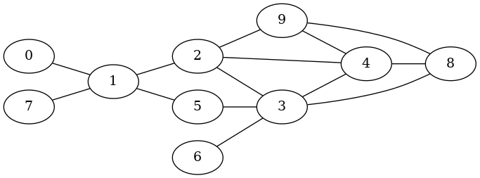
Next to our graph we create a list of attributes or context information:
>>> context = [1,1,0,1,1,1,1,0,1,0]
This is a very simple example of a bool-attriute associated with each node (the third entry in this list yields the attribute of the third vertex in g and so on).
The unique feature of nctx comes here: Define a function that is evaluated at each node during shortest path discovery. Therefore, the function has to accept three parameters: the start vertex, the current, and the next vertex. It must evaluate to bool in order to guide edge traversal.
>>> def decision(strt, crnt, nxt):
...     return context[crnt] == context[nxt]
Here, we use an edge only if its source and end vertex have the same context information assigned:
>>> path = nctx.AlgPaths.find_path_ctx(g, 0, 6, decision)
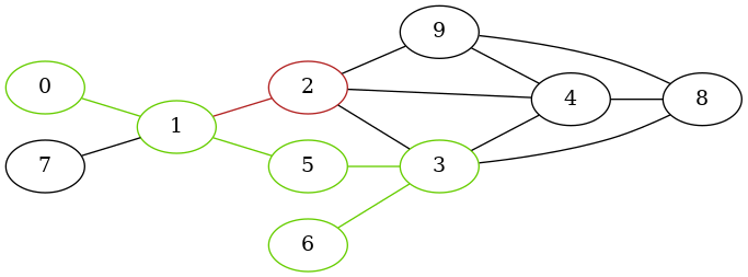
The shortest path from 0 to 6 is
>>> list(path)
[0, 1, 5, 3, 6]
For example, the edge 1 -> 2 was not visited because of contextual constraints: context[1] != context[2].
For this example of shortest path discovery from start to target, passing the start vertex to the decision function is unnecessary. However, the signature of this function is consistent for all shortest-path- and centrality-related functionality. It becomes clear for the discovery of all shortest paths in the network. Here, we need the start vertex to know the vertex for which shortest paths are discovered:
>>> distances = nctx.AlgPaths.dijkstra_apsp_ctx(g, decision)
The result is a distance matrix:
>>> for dists in distances:
...     [d if d < core.VecULong._max() else float("inf") for d in dists]
[0, 1, inf, 3, 4, 2, 4, inf, 4, inf]
[1, 0, inf, 2, 3, 1, 3, inf, 3, inf]
[inf, inf, 0, inf, inf, inf, inf, inf, inf, 1]
[3, 2, inf, 0, 1, 1, 1, inf, 1, inf]
[4, 3, inf, 1, 0, 2, 2, inf, 1, inf]
[2, 1, inf, 1, 2, 0, 2, inf, 2, inf]
[4, 3, inf, 1, 2, 2, 0, inf, 2, inf]
[inf, inf, inf, inf, inf, inf, inf, 0, inf, inf]
[4, 3, inf, 1, 1, 2, 2, inf, 0, inf]
[inf, inf, 1, inf, inf, inf, inf, inf, inf, 0]
Since the decision function receives IDs of vertices, we can complicate our attribute data structure to contain vectors for each vertex:
>>> import numpy as np
>>> np.random.seed(42)
>>> context = np.random.rand(10,100)
Then, the decision function needs to be adapted to this new data structure:
>>> def decision(strt, crnt, nxt):
...     return core.angular_distance(context[crnt], context[nxt]) <= core.angular_distance(context[strt], context[nxt])
This decision function makes use of built-in distance functions for numeric vectors (see nctx.core for more infos on these functions). Using this, we could evaluate the betweenness centrality, for example:
>>> betw_ctx = nctx.AlgCentralities.betweenness_ctx(g, decision)
It results in the following betweenness values for the vertices:
>>> list(betw_ctx)
[0.0, 0.0, 2.4583333333333335, 2.125, 0.9166666666666665, 0.0, 0.0, 0.0, 0.5, 0.5833333333333333]
More examples can be found in the documentation of the functions: